
Machine Learning for Trading (with Python)
The Rise Of The Machines In Search For Alpha
© Ran Aroussi
@aroussi | aroussi.com | github.com/ranaroussi
![]()
September, 2018
Agenda
- Machine Learning Overview
- The Machine Learning Workflow
- Common Machine Learning Algorithms
- ML Algorithms for Trading
- Example of a Trading Strategy that uses ML
- Further Reading


Machine Learning Overview
Machine Learning
What is Machine Learning?
Machine learning is the science of getting computers to act without being explicitly programmed. It uses statistical techniques to give computers the ability to "learn" from data.
* Note that ML research is a close neighbour of data mining, and hence overfitting is something you should pay very close attention to.
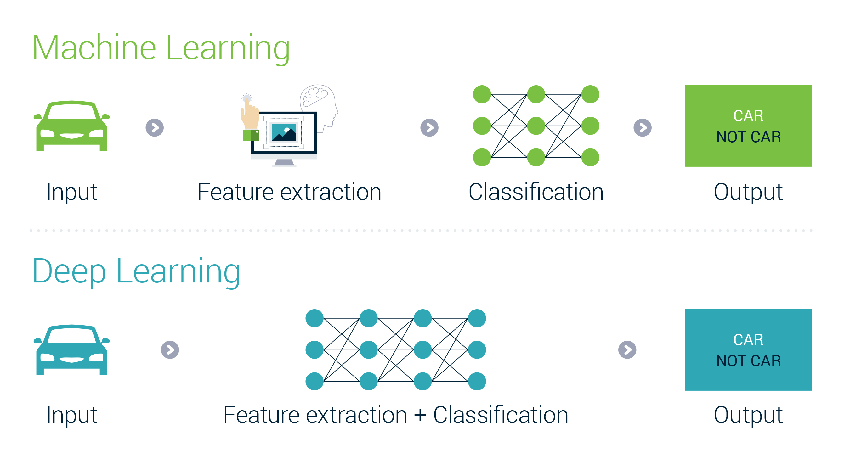
Maching Learning vs. Deep Learning
- Machine learning uses algorithms to parse data, learn from that data, and make informed decisions based on what it has learned.
- Deep learning structures algorithms in layers to create an “artificial neural network” that can learn and make intelligent decisions on its own.
Deep learning is a subfield of machine learning. While both fall under the broad category of artificial intelligence, deep learning is what powers the most human-like artificial intelligence.

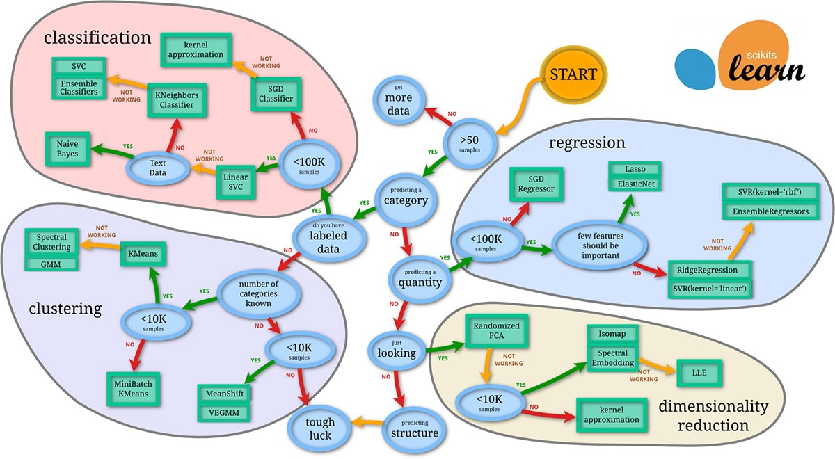
Machine Learning Algorithms
Machine Learning Algorithms
- Unupervised Learning: based on input
- Supervised Learning: based on input + output
- Reinforced Learning: based on feedback
- Deep Learning: based on nothing :)

The Machine Learning Workflow
The Machine Learning Workflow
- Data Gathering + Cleaning
- Feature Engineering + Normalization
- Model Selection
- Split Data
- Train Data
- Test Data
Feature Engineering ≈ Alpha Factors
Features are attributes that holds some predictive power over the end result
Examples:
- Previous N days returns
- Inter-market relationships
- Technical indicators
Machine Learning for Trading
Machine Learning for Trading
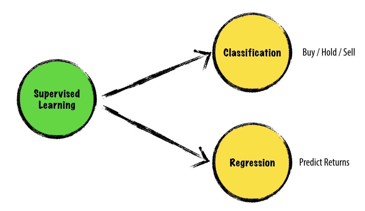
ML Algorithms for "Beginners"
The two ML algorithems that are easiest to get started with are Decision Trees and K Nearest-Neighbours. They are both easy to comprehend and works for either Regression or Classification.
KNN (K Nearest-Neighbours)
- Training is fast
- Query is slow
- Requires data normalization
- Needs features

Decision Trees
- Training is slow
- Query is fast
- No need for data normalization
- Auto-discover features
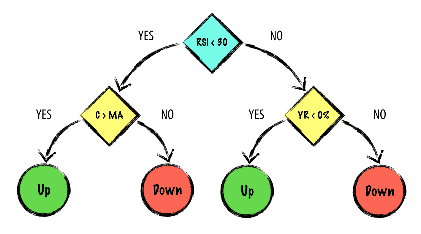
Example: Predicting Tomorrow's Direction using a Decision Tree Algorithm
In [3]:
from sklearn.tree import DecisionTreeClassifier
from sklearn import preprocessing
from sklearn.model_selection import cross_val_score
from sklearn.metrics import accuracy_score
Get Data
In [4]:
symbols = ["^GSPC", "^VIX", "^VXV"]
raw = pd.read_pickle('ml-raw-data.pkl')

df = pd.DataFrame()
for symbol in symbols:
    new_symbol = symbol.replace("^", "").replace("GSPC", "SPX")
    df[new_symbol] = raw[symbol]['Close']

df.tail()
Out[4]:
Prepare Features (input)
In [5]:
df['SPXVOL'] = raw['^GSPC']['Volume'].pct_change() * 100
df['SPX1D']  = raw['^GSPC']['Close'].pct_change() * 100
df['VIX1D']  = raw['^VIX']['Close'].pct_change() * 100
df['VXV1D']  = raw['^VXV']['Close'].pct_change() * 100

df['SPXHL']  = raw['^GSPC']['Open'] - raw['^GSPC']['Low']
df['SPXOC']  = raw['^GSPC']['Open'] - raw['^GSPC']['Close']
df['SPXO2C'] = ((raw['^GSPC']['Close'] / raw['^GSPC']['Open']) - 1) * 100

df.dropna(inplace=True)
df.tail()
Out[5]:
Prepare target (output)
In [6]:
df['target'] = np.where(df["SPXO2C"] >= 0, 1, np.where(df["SPXO2C"] < 0, -1, 0))
df['target'] = df['target'].shift(-1) # next day

df.dropna(inplace=True)
df.tail(10)
Out[6]:
Split Data into training and testing
In [7]:
feature_cols = [col for col in df.columns if col not in ['target']]

features = df[feature_cols].values
labels   = df['target'].values.flatten()

# split df
train_test_split = .9
sample = int( len(df.index) * train_test_split )

train_features = features[:-sample]
train_labels   = labels[:-sample]

test_features = features[-sample:]
test_labels   = labels[-sample:]
Normalize data
In [8]:
# normalize
normalizer = preprocessing.Normalizer()
train_features = normalizer.fit(train_features).transform(train_features)
Do ML Stuff
In [9]:
# init classifier
clf = DecisionTreeClassifier()

# fit
clf.fit(train_features, train_labels)
Out[9]:
In [10]:
# predict
prediction = clf.predict(test_features)

# score
accuracy_score(test_labels, prediction)
Out[10]:
In [11]:
scores = cross_val_score(clf, features, labels, cv=10)
print("Mean %.2f%%, Std: %.2f" % (scores.mean()*100, scores.std()*100) )
Test Strategy
In [12]:
testdf = df[-sample:].copy()
testdf['predicted'] = prediction

testdf.tail()
Out[12]:
In [13]:
testdf['strategy'] = testdf['predicted'].shift(1) * testdf['SPXO2C']

testdf[['SPX1D', 'strategy']].cumsum().plot()
Out[13]:

and... We're Done :)
This was the part 4 out of the 4-part webinar series
Prototyping Trading StrategiesBacktesting & OptimizationLive TradingUsing Machine Learning in Trading
Webinars available @ aroussi.com/webinars
Further Reading
Machine Learning for Trading (with Python)
Thank you for attending!
© Ran Aroussi
@aroussi | aroussi.com | github.com/ranaroussi
![]()
September, 2018